1 Introduction
Changes in climate conditions observed over the last few decades are considered to be the cause of change in magnitude and frequency of occurrence of extreme events (IPCC, 2013). The Fifth Assessment Report (AR5) of the Intergovernmental Panel on Climate Change (IPCC, 2013) has indicated a global surface temperature increase of 0.3 to 4.8 °C by the year 2100 compared to the reference period 1986-2005 with more significant changes in tropics and subtropics than in mid-latitudes. It is expected that rising temperature will have a major impact on the magnitude and frequency of extreme precipitation events in some regions (Barnett et al., 2006; Wilcox et al., 2007; Allan et al., 2008; Solaiman et al., 2011). Incorporating these expected changes in planning, design, operation and maintenance of water infrastructure would reduce unseen future uncertainties that may result from increasing frequency and magnitude of extreme rainfall events.
According to the AR5, heavy precipitation events are expected to increase in frequency, intensity, and/or amount of precipitation under changing climate conditions. Table 1 summarizes assessments made regarding heavy precipitation in AR5 (IPCC, 2013 – Table SPM.1).
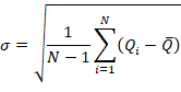
Table 1: Summary of AR5 assessments for extreme precipitation
|
Assessment that changes occurred since 1950 |
Assessment of a human contribution to observed changes |
Likelihood of further changes |
|
|
Early 21st century |
Late 21st century |
||
|
Likely more land areas with increases than decreases |
Medium Confidence |
Likely over many land areas |
Very likely over most of the mid-latitude land masses and over wet tropical areas |
|
Likely more land areas with increases than decreases |
Medium confidence |
Likely over many areas |
|
|
Likely over most land areas |
More likely than not |
Very likely over most land areas |
|
Since it is evident that the global temperature is increasing with climate change, it follows that the saturation vapor pressure of the air will increase, as it is a function of air temperature. Further, it is observed that the historical precipitation data has shown considerable changes in trends over the last 50 years (Figure 1 and Figure 2). These changes are likely to intensify with increases in global temperature (IPCC, 2013).
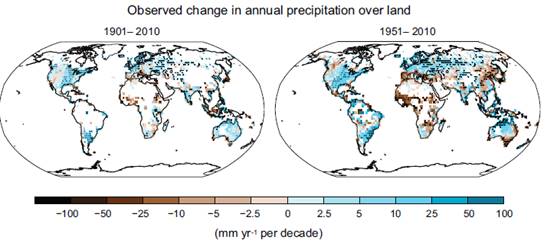
Figure 1: Chances in observed precipitation from 1901 to 2010 and from 1951 to 2010 (after IPCC, 2013)
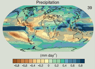
Figure 2: Changes in annual mean precipitation for 2081-2100 relative to 1986-2005 under Representative Concentration Pathway 8.5. (after IPCC, 2013)
Evaluation of change in precipitation intensity and frequency is critical as these data are used directly in design and operation of water infrastructure. However, practitioners’ application of climate change science remains a challenge for several reasons, including: 1) the complexity and difficulty of implementing climate change impact assessment methods, which are based on heavy analytical procedures; 2) the academic and scientific communities’ focus on publishing research findings under rigorous peer review processes with limited attention given to practical implementation of findings; 3) political dimensions of climate change issue; and 4) a high level of uncertainty with respect to future climate projections in the presence of multiple climate models and emission scenarios.
This project aimed to develop and implement a generic and simple tool to allow practitioners to easily incorporate impacts of climate change, in form of updated IDF curves, into water infrastructure design and management. To accomplish this task, a web-based tool was developed (referred to as the IDF_CC tool), consisting of a user-friendly interface with a powerful database system and sophisticated, but efficient, methodology for the update of IDF curves (Simonovic et al., 2016).
Intensity duration frequency (IDF) curves are typically developed by fitting a theoretical probability distribution to an annual maximum precipitation (AMP) time series. AMP data are fitted using extreme value distributions like Gumbel, Generalized Extreme Value (GEV), Log Pearson, Log Normal, among other approaches. IDF curves provide precipitation accumulation depths for various return periods (T) and different durations, usually, 5, 10, 15, 20 30 minutes, 1, 2, 6, 12, 18 and 24 hours. Durations exceeding 24 hours may also be used, depending on the application of IDF curves. Hydrologic design of storm sewers, culverts, detention basins and other elements of storm water management systems is typically performed based on specified design storms derived from IDF curves (Solaiman and Simonovic, 2010; Peck et al., 2012).
The IDF_CC tool version 3 adopts Gumbel distribution for fitting the historical AMP data and GEV distribution for fitting both historical and future precipitation data. The parameter estimation for the selected distributions is carried out using the method of moments for Gumbel and L-moments for GEV. Version 3 of the tool also introduces a new dataset of ungauged IDF curves for Canada. With the new module, users can obtain IDF curves for any location in the country, including regions where no observations are available (i.e., ungauged locations).
The web based IDF_CC tool is built as a decision support system (DSS). As such, it includes traditional DSS components: a user interface, database and model base.[1] One of the major components of the IDF_CC DSS is a model base that includes a set of mathematical models and procedures for updating IDF curves. These mathematical models are an important part of the IDF_CC tool and are used for the calculations required to develop IDF curves based on historical data and for updating IDFs to reflect future climatic conditions. The models and procedures used within the IDF_CC tool include:
• Statistical analysis algorithms: statistical analysis is applied to fit the selected theoretical probability distributions to both historical and future precipitation data. To fit the data, Gumbel and GEV distributions are used within the tool. They are fitted using method of moments and L-moments, respectively. The GCM data used in statistical analysis are spatially interpolated from the nearest grid points using the inverse distance method.
• Optimization algorithm: an algorithm used to fit the analytical relationship to an IDF curve.
• IDF update algorithm: the equidistant quantile matching (EQM) algorithm is applied to the IDF updating procedure.
This technical manual presents the details of the statistical analysis procedures and IDF update algorithm. For the optimization algorithm, readers are referred to UserMan Appendix A.
2 Background
2.1 Intensity-Duration-Frequency Curves
Reliable rainfall intensity estimates are necessary for hydrologic analyses, planning, management and design of water infrastructure. Information from IDF curves is used to describe the frequency of extreme rainfall events of various intensities and durations. The rainfall IDF curve is one of the most common tools used in urban drainage engineering, and application of IDF curves for a variety of water management applications has been increasing (CSA, 2012). The guideline Development, Interpretation and Use of Rainfall Intensity-Duration-Frequency (IDF) Information: A Guideline for Canadian Water Resources Practitioners, developed by the Canadian Standards Association (CSA, 2012), lists the following reasons for increasing application of rainfall IDF information:
· As the spatial heterogeneity of extreme rainfall patterns becomes better understood and documented, a stronger case is made for the value of “locally relevant” IDF information.
· As urban areas expand, making watersheds generally less permeable to rainfall and runoff, many older water systems fall increasingly into deficit, failing to deliver the services for which they were designed. Understanding the full magnitude of this deficit requires information on the maximum inputs (extreme rainfall events) with which drainage works must contend.
· Climate change will likely result in an increase in the intensity and frequency of extreme precipitation events in most regions in the future. As a result, IDF values will optimally need to be updated more frequently than in the past and climate change scenarios might eventually be drawn upon in order to inform IDF calculations.
The typical development of rainfall IDF curves involves three steps. First, a probability distribution function (PDF) or Cumulative Distribution Function (CDF) is fitted to rainfall data for a number of rainfall durations. Second, the maximum rainfall intensity for each time interval is related with the corresponding return period from the CDF. Third, from the known cumulative frequency and given duration, the maximum rainfall intensity can be determined using an appropriate fitted theoretical distribution function (such as GEV, Gumbel, Pearson Type III, etc.) (Solaiman and Simonovic, 2010).
2.2 Updating IDF Curves
The main assumption in the process of developing IDF curves is that the historical series are stationary and therefore can be used to represent future extreme conditions. This assumption is not valid under rapidly changing conditions, and therefore IDF curves that rely only on historical observations will misrepresent future conditions (Sugahara et al., 2009; Milly et al., 2008). Global Climate Models (GCMs) are one of the best ways to explicitly address changing climate conditions for future periods (i.e., non-stationary conditions). GCMs simulate atmospheric patterns on larger spatial grid scales (usually greater than 100 kilometers) and are therefore unable to represent the regional scale dynamics accurately. In contrast, regional climate models (RCMs) are developed to incorporate the local-scale effects and use smaller grid scales (usually 25 to 50 kilometers). The major shortcoming of RCMs is the computational requirements to generate realizations for various atmospheric forcings.
Both GCMs and RCMs have larger spatial scales than the size of most watersheds, which is the relevant scale for IDF curves. Downscaling is one of the techniques to link GCM/RCM grid scales and local study areas for the development of IDF curves under changing climate conditions. Downscaling approaches can be broadly classified as either dynamic or statistical. The dynamic downscaling procedure is based on limited area models or uses higher resolution GCM/RCM models to simulate local conditions, whereas statistical downscaling procedures are based on transfer functions which relate GCM outputs with the local study areas; that is, a mathematical relationship is developed between GCM outputs and historically observed data for the time period of observations. Statistical downscaling procedures are used more widely than dynamic models because of their lower computational requirements and availability of GCM outputs for a wider range of emission scenarios. Table 2 provides comparison between dynamic downscaling and statistical downscaling.
Table 2: Comparison of dynamic downscaling and statistical downscaling
|
Criteria |
Dynamic downscaling |
Statistical downscaling |
|
Computational time |
Slower |
Fast |
|
Experiments |
Limited realizations |
Multiple realizations |
|
Complexity |
More complete physics |
Succinct physics |
|
Examples |
Regional climate models, Nested GCMs |
Linear regression, Neural network, Kernel regression |
The IDF_CC tool version 3 adopts a modified version of the equidistant quantile-matching (EQM) method for temporal downscaling of precipitation data developed by Srivastav et al. (2014), which can capture the distribution of changes between the projected time period and the baseline. Future projections are incorporated by using the concept of quantile delta mapping (Olsson et al., 2012; and Cannon et al., 2015), also known as scaling. For spatial downscaling, version 3 of the tool utilizes data from GCMs produced for Coupled Model Intercomparison Project Phase 5 - CMIP5 (IPCC, 2013) and statistically downscaled daily Canada-wide climate scenarios, at a gridded resolution of 300 arc-seconds (0.0833 degrees, or roughly 10 km) for the simulated period of 1950-2100 (PCIC, 2013). Spatially and temporally downscaled information is used for updating IDF curves.
2.2.1 Gauged locations
In the case of the EQM method for gauged locations, the quantile-mapping functions are directly applied to annual maximum precipitation (AMP) to establish statistical relationships between the AMPs of GCM and sub-daily observed (historical) data rather than using complete daily precipitation records. In terms of modelling complexity, this methodology is relatively simple and computationally efficient. Figure 3 explains a simplified approach for using the EQM method combined with statistically downscaled daily Canada-wide climate scenarios. The three main steps that are involved in using EQM method are: (i) establishment of statistical relationship between the AMPs of the GCM baseline (or modeled historical) and the observed station of interest, which is referred to as temporal downscaling (See Figure 3 brown dashed arrow); and (ii) establishment of statistical relationship between the AMPs of the base period GCM and the future period GCM, which is referred as scaling or quantile delta mapping (see Figure 3 black arrow); and (iii) establishment of statistical relationship between steps (i) and (ii) to update the IDF curves for future periods (See Figure 3 red arrow). For a detailed description of the methodology see Section 4.2 of the current document.
![]()
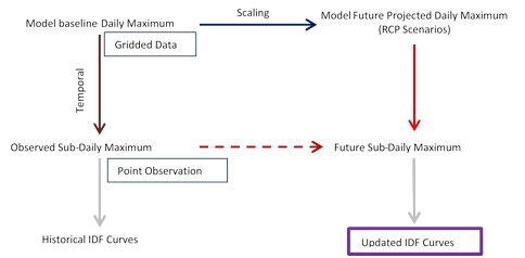
Figure 3: Concept of equidistance quantile matching method for updating IDF curves for gauged locations
2.2.2 Ungauged locations
For the ungauged locations an adaptation of the EQM method is necessary. In this case, the ungauged IDF curve estimates, for all durations (5, 10, 15, 30 min, 1, 2, 6, 12 and 24 hrs) and return periods (2, 5, 10, 25, 50 and 100 years), are extracted directly from the gridded dataset produced for the IDF_CC tool and described in detail in Item 3.3. Figure 4 explains a simplified approach for using the modified EQM method with the three main steps:(i) establishment of statistical relationship between the AMPs of the base period GCM and the future period GCM, which is referred as scaling or quantile delta mapping (see Figure 4 dark blue arrow); and (ii) establishment of statistical relationship between IDF estimate for the ungauged location selected, and the steps (i) to update the IDF curves for future periods (See Figure 4 brown dashed and red arrows). For a detailed description of the methodology see Section 6.3 of the current document.
![]()
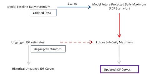
Figure 4: Concept of the modified equidistance quantile matching method for updating IDF curves for ungauged locations
2.3 Global Climate Models (GCMs) and Representative Concentration Pathways (RCPs)
GCMs represent dynamics within the Earth’s atmosphere for the purposes of understanding current and future climatic conditions. These models are the best tools for assessment of the impacts of climate change. There are numerous GCMs developed by different climate research centres. They are all based on (i) land-ocean-atmosphere coupling; (ii) greenhouse gas emissions, and; (iii) different initial conditions representing the state of the climate system. These models simulate global climate variables on coarse spatial grid scales (e.g., 250 km by 250 km) and are expected to mimic the dynamics of regional-scale climate conditions. GCMs are extended to predict the atmospheric variables under the influence of climate change due to global warming. The amount of greenhouse gas emissions is the key variable for generating future scenarios. Other factors that may influence the future climate include land-use, energy production, global and regional economy and population growth.
To update IDF curves under changing climatic conditions, the IDF_CC tool version 3 uses 24 GCMs from different climate research centers (see UserMan: Section 3.3) and 9 GCMs downscaled using the Bias Correction/Constructed Analogues with Quantile mapping reordering (BCCAQ) method, which results in 33 GCM datasets. These model outputs are available in the netCDF format that is widely used for storing climate data. The IDF_CC tool converts the netCDF files into a more efficient format to reduce storage space and computational time. These converted climate data files are stored in the IDF_CC tool’s database (see UserMan: Section 1.2). Salient features of each of the GCMs used in the IDF_CC tool are presented in Appendix A. The data for the various GCMs can be downloaded from https://esgf-node.llnl.gov/projects/esgf-llnl/ and http://tools.pacificclimate.org/dataportal/downscaled_gcms/map/, which are gateways for scientific data collections. These models are adopted based on the availability of complete sets of future greenhouse gas concentration scenarios, also known as Representative Concentration Pathways (RCPs), which are described in detail in the IPCC AR5 report (See: IPCC Fifth Assessment Report – Annex 1 Table: AI.1), and briefly described below.
Because updating IDF curves using all of the time series for each of the downscaled GCMs would be demanding for the user, the IDF_CC tool provides two options (UserMan: Section 3.4), including: (i) selection of any model from the list of GCMs provided with the tool or (ii) selection of model ensemble. The users are encouraged to test different models due to the uncertainty associated with climate modeling (UserMan: Section 3.4).
The Fifth Assessment Report (AR5) of the Intergovernmental Panel on Climate Change (IPCC, 2013) introduced new future climate scenarios associated with RCPs), which are based on time-dependent projections of atmospheric greenhouse gas (GHG) concentrations. RCPs are scenarios that include time series of emissions and concentrations of the full suite of greenhouse gases, aerosols and chemically active gases, as well as land use and land cover factors (Moss et al., 2008). The word “representative” signifies that each RCP provides only one of many possible scenarios that would lead to the specific radiative forcing[2] characteristics. The term “pathway” emphasizes that not only the long-term concentration levels are of interest, but also the trajectory taken over time to reach that outcome (Moss et al., 2010).
There are four RCP scenarios: RCP 2.6, RCP 4.5, RCP 6.5 and RCP 8.5. The following definitions are adopted directly from IPCC AR5 (IPCC, 2013):
· RCP2.6: One pathway where radiative forcing peaks at approximately 3 W m–2 before 2100 and then declines (the corresponding Extended Concentration Pathways[3] (ECP) assuming constant emissions after 2100).
· RCP4.5 and RCP6.0: Two intermediate stabilization pathways in which radiative forcing is stabilized at approximately 4.5 W m–2 and 6.0 W m–2 after 2100 (the corresponding ECPs assuming constant concentrations after 2150).
· RCP8.5: One high pathway for which radiative forcing reaches greater than 8.5 W m–2 by 2100 and continues to rise for some time (the corresponding ECP assuming constant emissions after 2100 and constant concentrations after 2250).
The future emission scenarios used in the IDF_CC tool are based on RCP 2.6, RCP 4.5 and RCP 8.5 (UserMan: Section 3.2 and 3.3). RCP 2.6 represents the lower emission scenario, followed by RCP 4.5 as an intermediate level and RCP 8.5 as the higher emission scenario. IDF curves developed using all three RCPs represent the range of uncertainty or possible range of IDF curves under changing climatic conditions. The IDF_CC tool has two representations of future IDF curves (UserMan: Section 3.3): (i) updated IDF curve for each RCP scenario – each IDF curve is averaged from all the GCMs and all emission scenarios; and (ii) comparison of future and historical IDF curves.
2.4 Bias Correction
The IDF_CC tool database incorporates 9 bias corrected GCMs by the Bias Correction/Constructed Analogues with Quantile mapping reordering (BCCAQ) method (PCIC, 2013). The models were selected based on the availability of projections (RCP 2.6, 4.5 and 8.5). For each model, two bias corrected diverted datasets are available from PCIC (2013). Three additional downscaled GCMs are available from PCIC for RCP 4.5 and RCP 8.5 only. These models are not included with the IDF_CC tool.
The BCCAQ is a hybrid method that combines results from BCCA (Maurer et al., 2010) and quantile mapping (QMAP) (Gudmundsson et al., 2012). This method uses similar spatial aggregation and quantile mapping steps as Bias-Correction Spatial Disaggregation - BCSD (Wood et al., 2004, Maurer et al., 2008 and Werner, 2011), but obtains spatial information from a linear combination of historical analogues for daily large-scale fields, avoiding the need for monthly aggregates (PCIC, 2013). QMAP applies quantile mapping to daily climate model outputs that have been interpolated to the high-resolution grid using the climate imprint method of Hunter and Meentemeyer (2005). BCCAQ combines outputs from these two methods. For more information on BCCAQ, refer to https://pacificclimate.org/data/statistically-downscaled-climate-scenarios and Werner and Cannon (2015).
2.5 Selection of GCMs
According to the fifth assessment report of IPCC, there are 42 GCMs developed by various research centres (Table AI.1 from Annex I, IPCC AR5). The IDF_CC tool adopts only 24 GCMs out of the 42 listed GCMs because: i) not all the GCMs provide simulation results for the three selected RCPs for future climate scenarios (i.e., RCP 2.6, 4.5 and 8.5); and ii) there are some technical limitations related to downloading the data for some GCMs, including connection to remote servers or repositories for GCM datasets.
Currently, the IDF_CC tool uses 24 GCMs from IPCC AR5 (raw datasets) and 9 bias-corrected GCMs using the BCCAQ method (Section 2.4). These datasets are selected based on the availability of all three future climate scenarios for updating the IDF curves (UserMan: Section 3.3). IDC_CC tool users can select any individual GCM data set or ensemble of all available raw and bias corrected models.
Users should note that the climate modelling community does not “compare” global climate models to identify superior/inferior models for specific locations. Thus, users should note that there is no “right” GCM for any given location. Users are provided access to all available models in the IDF_CC tool to allow them to understand uncertainty associated with potential climate change impacts.
2.6 Historical Data
With respect to historical data, the IDF_CC tool contains a repository of Environment and Climate Change Canada stations. Further, the user can provide their own dataset and develop historical and future IDF curves. For more detail on how to use user-defined historical datasets, refer to UserMan: Section 2.5. Historical datasets used with the IDF_CC tool for development of future IDF curves must satisfy the following conditions:
1. Data length: The minimum length of the historical data to calculate the IDF curves should be equal to, or greater, than 10 years (the minimum value used by Environment and Climate Change Canada to develop IDF curves), and
2. Missing Values: The IDF_CC tool does not infill and/or extrapolate missing data. The user should provide complete data without missing values.
3 Methodology
The mathematical models of the IDF_CC tool provide support for calculations required to develop IDF information based on historical data for the gauged locations, IDF information for ungauged locations, and GCM outputs. Models and procedures used within the IDF_CC tool include:
(i) statistical analysis for fitting Gumbel distribution using the method of moments and inverse distance method for spatial interpolation (UserMan: Section 3.1);
(ii) statistical analysis for fitting GEV distribution using the L-moments method (UserMan: Section 3.1); and
(iii) IDF updating algorithms for future climate change scenarios for both gauged and ungauged locations (UserMan: Section 3.3 and 3.4).
The next two sections present the algorithms for both modules (IDF information for gauged and ungauged locations) and their implementation with the IDF_CC tool are presented.
Implementation of each algorithm is illustrated using a simple example in this section. The example uses historical observed data from Environment and Climate Change Canada for a London, Ontario station and GCM data for the base period and future time period from the downscaled Canadian GCM CanESM2 using the BCCAQ method, spatially interpolated to the London station. The data is presented in Appendix B. For simplicity, the examples use 5-minute annual maximum precipitation. The same procedure can be followed for other durations.
The Gumbel and GEV probability distributions are adopted for use by the IDF_CC tool. They have a wide variety of applications for estimating extreme values of given data sets, and are commonly used in hydrologic applications. They are used to generate the extreme precipitation at higher return periods for different durations (UserMan: Section 3.1 and 3.2). The statistical distribution analysis is a part of the mathematical models used with the IDF_CC tool (UserMan: Section 1.4). The following sections explain the theoretical details of the statistical analyses implemented with the tool.
3.1 Common Methods
This section describes the methods used by the IDF_CC tool to fit and update the IDF curves. The Gumbel and GEV distributions are briefly presented, followed by the parameter estimation procedures. For Gumbel the method of Moments is used and for GEV, the method of L-Moments is used. The spatial interpolation procedure is used in the updating methods to spatially downscale GCM data for selected gauged and ungauged locations.
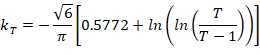
3.1.1 Gumbel Distribution (EV1)
The EV1 distribution has been widely recommended and adopted as the standard distribution by Environment and Climate Change Canada for all Precipitation Frequency Analyses in Canada. The EV1 distribution for annual extremes can be expressed as:
|
|
Eq. 1 |
where Q(x) is the exceedance value, µ
and ![]() are the population mean and standard deviation of the
annual extremes; T is return period in years.
are the population mean and standard deviation of the
annual extremes; T is return period in years.
|
|
Eq. 2 |
3.1.2 Generalized Extreme Value (GEV) Distribution
The GEV distribution is a family of continuous probability distributions that combines the three asymptotic extreme value distributions into a single one: Gumbel (EV1), Fréchet (EV2) and Weibull (EV3) types. GEV uses three parameters: location, scale and shape. The location parameter describes the shift of a distribution in each direction on the horizontal axis. The scale parameter describes how spread out the distribution is and defines where the bulk of the distribution lies. As the scale parameter increases, the distribution will become more spread out. The shape parameter affects the shape of the distribution and governs the tail of each distribution. The shape parameter is derived from skewness, as it represents where most of the data lies, which creates the tail(s) of the distribution. A value of shape parameter k = 0 indicates an EV1 distribution. A value of k > 0, indicates EV2 (Fréchet), and k < 0 indicates the EV3 distribution (Weibull). The Fréchet type has a longer upper tail than the Gumbel distribution and the Weibull type has a shorter tail (Overeem et al., 2007; and Millington et al., 2011).
The GEV cumulative
distribution function F(x) is given by Eq. 3 for k ![]() 0
and Eq. 4 for k = 0
(EV1).
0
and Eq. 4 for k = 0
(EV1).
|
|
Eq. 3 |
|
|
Eq. 4 |
with µ the location, ![]() the
scale and k the shape parameter of the distribution, and y the Gumbel
reduced variate,
the
scale and k the shape parameter of the distribution, and y the Gumbel
reduced variate, ![]() .
.
The inverse distribution function or quantile function is given by Eq. 5 for k ≠ 0 and Eq. 6 for k = 0.
|
|
Eq. 5 |
|
|
Eq. 6 |
3.1.3 Parameter Estimation Methods
A common statistical procedure for estimating distribution parameters is the use of a maximum likelihood estimator or the method of moments. Environment and Climate Change Canada uses and recommends the use of the method of moments technique to estimate the parameters for EV1. The IDF_CC tool uses the method of moments to calculate the parameters of the Gumbel distribution (UserMan: Section 1.4 and 3.1). The tool uses L-moments to calculate parameters of the GEV distribution (see UserMan. Sections 1.4 and 3.1). The following sections describe the method of moments procedure for calculating the parameters of the Gumbel distribution and L-moments method for calculating parameters of the GEV distribution.
3.1.3.1 Method of Moments for Gumbel
The most popular method for estimating the parameters of the Gumbel distribution is method of moments (Hogg et al., 1989). In the case of the Gumbel distribution, the number of unknown parameters is equal to the mean and standard deviation of the sample mean. The first two moments of the sample data will be sufficient to derive the parameters of the Gumbel distribution in Eq. 7 and Eq. 8. These are defined as:
|
|
Eq. 7 |
|
|
Eq. 8 |

Where ![]() is the mean,
is the mean, ![]() the value of standard deviation of the historical
data,
the value of standard deviation of the historical
data, ![]() the maximum precipitation data for year i, and
the maximum precipitation data for year i, and
![]() the mean.
the mean.
|
Example: 3.1 The step-by-step procedure followed by IDF_CC tool (UserMan: Section 3.1) for the estimation of the Gumbel distribution (EV1) parameters is: 1. Calculate the mean of the historical data using Eq. 7:
2. Calculate the value of standard deviation of the historical data using Eq. 8:
3. Calculate the value of KT for a given return period (assuming return period (T) equal to 100 years) using Eq. 2:
4. Calculate the precipitation for a given return period using Eq. 1:
5. Finally, the precipitation intensities are calculated for different return periods and frequencies. The IDF curves using the Gumbel distribution for the historical data are obtained as:
|
|||||||||||||||||||||||||||||||||||||||||||||||||||||||||||||||||||||||||||||
3.1.3.2 L-moments Method for GEV
The L-moments (Hosking et al., 1985; and Hosking and Wallis, 1997) and maximum likelihood methods are commonly used to estimate the parameters of the GEV distribution and fit to annual maxima series. L-moments are a modification of the probability-weighted moments (PWMs), as they use the PWMs to calculate parameters that are easier to interpret. They PMWs can be used in the calculation of parameters for statistical distributions (Millington et al., 2011). They provide an advantage, as they are easy to work with, and more reliable as they are less sensitive to outliers. L-moments are based on linear combinations of the order statistics of the annual maximum rainfall amounts (Hosking et al., 1985; and Overeem et al., 2007). The PWMs are estimated by:
|
|
Eq. 9 |
|
|
Eq. 10 |
|
|
Eq. 11 |
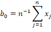
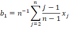
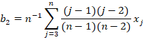
where xj is the ordered sample of annual maximum series (AMP) and bi are the first PWMs. The sample L-moments can them obtained as:
|
|
Eq. 12 |
|
|
Eq. 13 |
|
|
Eq. 14 |
The GEV parameters:
location (µ), scale (![]() )
and shape (k) are defined (Hosking and Wallis, 1997) as:
)
and shape (k) are defined (Hosking and Wallis, 1997) as:
|
where:
|
Eq. 15 |
|
|
Eq. 16 |
|
|
Eq. 17 |
where ![]() is the gamma function,
is the gamma function, ![]() ,
, ![]() and
and
![]() the
L-moments, and µ the location,
the
L-moments, and µ the location, ![]() the scale and k the shape parameters of the GEV
distribution.
the scale and k the shape parameters of the GEV
distribution.
|
Example: 3.2 The step-by-step procedure followed by the IDF_CC tool (UserMan: Section 3.1) for the estimation of the GEV distribution parameters includes: 1. Sort the AMP in the ascending order 2. Calculate the PWMs of the historical data using Eq. 9, Eq. 10 and Eq. 11:
3. Calculate the value of the L-moments using Eq. 12, Eq. 13 and Eq. 14:
4. Calculate the GEV parameters using Eq. 15, Eq. 16 and Eq. 17:
5. Calculate the precipitation for a given return period (assuming return period (T) equal to 100 years for the example bellow) using Eq. 6:
6. Finally, the precipitation intensities are calculated for different return periods and frequencies. The IDF curves using the GEV distribution with the historical data are obtained as:
|
|||||||||||||||||||||||||||||||||||||||||||||||||||||||||||||||||||||||||||||
3.1.4 Spatial Interpolation of the GCM data
The GCM data must be spatially interpolated to the station coordinates in order to be applied in the IDF_CC tool. The tool uses an inverse square distance weighting method, in which the nearest four grid points to the station are weighted by an inverse distance function from the station to the grid points (UserMan: Section 3.3). In this way, the grid points that are closer to the station are weighted more than the grid points further away from the station. The mathematical expression for the inverse square distance weighting method is given as:
|
|
Eq. 18 |
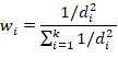
where di is the distance between the ith GCM grid point and the station, k is the number of nearest grid points - equal to 4 in the IDF_CC tool.
|
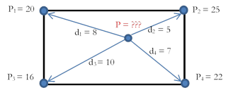
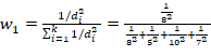
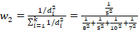
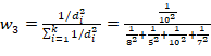
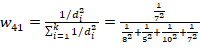
Example: 3.3 A hypothetical example shows calculation of spatial interpolation using inverse distance method. In this example, the historical observation station lies within four grid points. The procedure followed within the IDF_CC tool for the inverse distance method is as follows:
1. Calculate the weights using inverse distance method using Eq. 18:
2. Calculate the spatially interpolated precipitation using the above weights
= 20 x 0.167286 + 25 x 0.428253 + 16 x 0.107063 + 22 x 0.297398 = 22.30781 |
3.2 IDF Curves for Gauged Locations
The IDF_CC tool utilizes the Gumbel and GEV distribution functions and the parameter estimation methods described in Section 3 to fit the IDF curves for Gauged locations. The locations are the pre-loaded stations from Environment and Climate Change Canada, or the stations with user-provided data.
When the user requests to view an IDF for a station, the IDF_CC tool triggers a calculation process using the mathematical models in the background (please refer to UserMan Section 3.1 for more detail). The data analysis steps are as follows:
1) Read and organize data from the database for the selected station,
2) Data analysis (ignore negative and zero values) and extraction of yearly maximums,
3) Calculate statistical distributions parameters for GEV and Gumbel using L-moments and method of moments, respectively,
4) Calculate IDF curves as presented in examples on item 3.1 and 3.2, and
5) Fit interpolated equations to the IDF curve using optimization algorithm (Differential Evolution).
Data are then organized for for display (tables, plots, and equations - please refer to UserMan Section 3.1 for more detail).
3.3 IDF Curves for Ungauged Locations
A new dataset of ungauged rainfall IDFs was produced in included in the IDF_CC tool’s database allowing the development of IDF curves for ungauged locations across Canada. The methodology used in this study is similar to the methodology used in Faulkner and Prudhomme (1998) wherein first preliminary ungauged IDF estimates are made, followed by the correction of spatial errors in the estimates. The procedure for making preliminary IDF estimates in the IDF_CC tool is different from Faulkner and Prudhomme (1998) as estimates are made using Atmospheric Variables (AVs). AVs govern extreme precipitation development in different regions of Canada.
3.3.1 Preparation of predictors
Daily time-series of AVs listed in Table 3 are extracted for all grids located within Canada for the period 1979-2013 from both NARR (North American Regional Reanalysis), produced by the National Centers for Environmental Prediction (NCEP) and ERA-Interim, produced by European Centre for Medium-Range Weather Forecasts (ECMRWF) databases. Extracted time-series are used to calculate annual mean and maximum AV values to obtain an array of 31 predictors at all reanalysis grid-points. These values are used in step 3.4 when prediction of preliminary IDF estimates is made. Additionally, calculated predictors are bilinearly interpolated to obtain predictor values at all precipitation gauging station locations. These values are used in steps 3.2 and 3.3 to identify relevant AVs and to calibrate machine learning algorithms at each precipitation gauging station location.
3.3.2 Identification of Relevant AVs at Precipitation Gauging Station Locations
AVs governing AMP magnitudes (relevant AVs hereafter) are obtained using predictor variables calculated at different precipitation gauging stations for all stations with at least 10 years of data. Different sets of relevant AVs are obtained for AMPs of different precipitation durations. Since annual mean precipitation (P-mean) has been identified as an important predictor when modelling precipitation extremes (Faulkner and Prudhomme 1998; Van de Vyver 2012), it is considered as ‘reference’ predictor in this study. This means that P-mean is considered as one of the relevant predictors at all precipitation gauging stations.
The relevance of other AVs towards shaping AMP magnitudes is evaluated at each precipitation gauging station by performing chi-squared test and correlation analysis. The chi-squared test is performed to compare two nested linear regression models modelling observed AMP magnitudes: 1) model with only ‘reference’ predictor, and 2) model with ‘reference’ and a ‘test’ predictor. It is ascertained if the inclusion of the ‘test’ predictor variable leads to a statistically significant improvement (at p = 0.05) in the definition of model #1 or not. AVs resulting in a statistically significant improvement in regression model definition are also identified as relevant predictor variables. In addition, correlations between AMP and different AVs and extreme precipitation magnitudes are calculated and highly correlated AVs are also considered for modelling AMP magnitudes.
3.3.3 Calibration of machine learning (ML) models at precipitation gauging stations
ML models describing AMP magnitudes as a function of identified relevant AVs are calibrated at each precipitation gauging station. Different ML models are calibrated for different durations. To minimize the risk of obtaining unstable regression relationships at stations with short data lengths, observational and AV data from neighboring stations falling within a pooling extent are pooled when forming a relationship between AMP and relevant AVs. In this study, two pooling extents encompassing the 10 and 25 closest stations surrounding the gauging station of interest are considered for analysis. One machine learning algorithm, SVM (support vector machines) (Cortes and Vapnik 1993), is used to define the relationship between predictant and predictor variables. The kernlab package in R (https://cran.r-project.org/web/packages/kernlab/) is used to perform SVM modelling.
3.3.4 Prediction of preliminary IDF estimates at reanalysis grids
Prediction of preliminary IDF estimates for a particular reanalysis grid is made by using calibrated ML model from the nearest precipitation gauging station and time-series of predictors associated with the reanalysis grid as calculated in step 3.3.1. This process is repeated for all reanalysis grids and precipitation durations to obtain ungauged AMP estimates across Canada. Obtained AMP estimates are fitted to a Generalized Extreme Value (GEV) distribution and precipitation intensities corresponding to 2, 5, 10, 25, 50, and 100 year return periods are estimated.
3.3.5 Correction of spatial errors
Estimated preliminary IDF magnitudes are bilinearly
interpolated at precipitation gauging station locations. These preliminary
magnitudes are used in conjunction with IDF magnitudes obtained from
observational records to obtain correction factors at each precipitation
gauging station location. Different sets of correction factors are calculated
for IDFs of different durations and return periods. Correction factor ![]() obtained at a gauging station s, for a
precipitation event of duration d, and frequency f is calculated
as:
obtained at a gauging station s, for a
precipitation event of duration d, and frequency f is calculated
as:
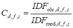 (8)
(8)
where subscripts obs and mod denote observed and modelled data respectively.
Correction factors calculated at each precipitation gauging station are bilinearly interpolated to obtain gridded correction factors for all reanalysis grids located within Canada. Correction factors obtained for reanalysis grids are multiplied with preliminary IDF estimates to obtain final ungauged IDF estimates.
Table 3. Atmospheric variables considered for the modelling of precipitation extremes in this study.
|
Predictor No. |
Atmospheric variable |
Predictor variables short-name |
|
1-2 |
AT-mean, AT-max |
|
|
3 |
Precipitation |
P-mean |
|
Downward shortwave radiative flux (surface) |
DSWRF-mean, DSWRF-max |
|
|
6-11 |
Geopotential height (1000 hpa, 850 hpa, 500 hpa) |
HGT1000hpa-mean, HGT1000hpa-max, HGT850hpa-mean, HGT850hpa-max, HGT500hpa-mean, HGT500hpa-max |
|
12-13 |
Total cloud cover |
TCC-mean, TCC-max |
|
14-15 |
WND-mean, WND-max |
|
|
16-21 |
Specific humidity (1000 hpa, 850 hpa, 500 hpa) |
SHUM1000hpa-mean, SHUM1000hpa-max, SHUM850hpa-mean, SHUM850hpa-max, SHUM500hpa-mean, SHUM500hpa-max |
|
22-23 |
MSLP-mean, MSLP-max |
|
|
24-25 |
CAPE-mean, CAPE-max |
|
|
26-31 |
Vertical velocity (1000 hpa, 850 hpa, 500 hpa) |
OMEGA1000hpa-mean, OMEGA1000hpa-max, OMEGA850hpa-mean, OMEGA850hpa-max, OMEGA850hpa-mean, OMEGA850hpa-max |
4 Updating IDF Curves Under a Changing Climate
The updating procedure for IDF curves is another component of the IDF_CC tool’s mathematical model base (UserMan: Section 1.4). There are two methods for updating IDF curves that differ depending on the type of analysis selected: 1) updating IDFs for gauged locations (either from existing stations provided by Environment and Climate Change Canada or stations created by the user; and 2) updating IDFs for ungauged locations from the gridded dataset. The methods are described here.
4.1 Updating IDFs for Gauged Locations
The tool uses an equidistant quantile matching (EQM) method to update IDF curves under changing climate conditions (UserMan: Section 3.3) by temporally downscaling precipitation data to explicitly capture the changes in GCM data between the baseline period and the future period. The flow chart of the EQM methodology is shown in Figure 5.

Figure 5: Equidistance Quantile-Matching method for generating future IDF curves under climate change
Equidistance Quantile Matching Method
The following section presents the EQM method for
updating the IDF curves that is employed by the IDF_CC tool version 3. The following
notation is used in the descriptions of the EQM steps: ![]() , stands for the annual maximum precipitation, j
is the subscript for 5min, 10min, 15min, 1hr, 2hr, 6hr, 12hr, 24hr sub-daily
durations, o the observed historical series, h for historical simulation
period (base-line for model data), m for model (downscaled GCMs), f
the sub/superscript for the future projected series, F the CDF of the
fitted probability GEV distribution and F-1 the inverse CDF. The
steps involved in the algorithm are as follows:
, stands for the annual maximum precipitation, j
is the subscript for 5min, 10min, 15min, 1hr, 2hr, 6hr, 12hr, 24hr sub-daily
durations, o the observed historical series, h for historical simulation
period (base-line for model data), m for model (downscaled GCMs), f
the sub/superscript for the future projected series, F the CDF of the
fitted probability GEV distribution and F-1 the inverse CDF. The
steps involved in the algorithm are as follows:
(i)
Extract sub-daily
maximums ![]() from the observed data at a given location (i.e.,
maximums of 5min, 10min, 15min, 1hr, 2hr, 6hr, 12hr, 24hr precipitation data) (UserMan:
Section 3.1).
from the observed data at a given location (i.e.,
maximums of 5min, 10min, 15min, 1hr, 2hr, 6hr, 12hr, 24hr precipitation data) (UserMan:
Section 3.1).
(ii)
Extract daily maximums for
the historical baseline period from the selected GCMs (UserMan: Section
3.2), ![]() .
.
(iii)
Fit the GEV probability
distribution to maxima series extracted in (i) for each sub-daily duration, ![]() , and for the GCM series from step (ii),
, and for the GCM series from step (ii), ![]() .
.
(iv)
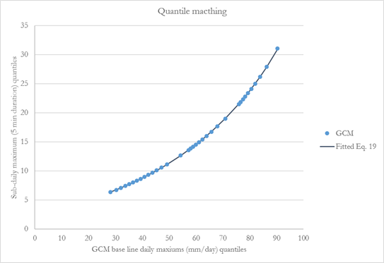
Based on sampling
technique proposed by Hassanzadeh et al. (2014), generate random numbers for non-exceedance
probability in the [0, 1] range. The quantiles extracted from the GEV fitted to
each pair ![]() and
and ![]() are equated to establish a statistical relationship
in the following form:
are equated to establish a statistical relationship
in the following form:
|
|
Eq. 19 |
where ![]() corresponds to the AMP
quantiles at the station scale
and
corresponds to the AMP
quantiles at the station scale
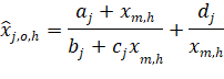
and ![]() , are the adjusted coefficients of the equation for
each sub-daily duration j. A Differential Evolution (DE) optimization algorithm
is used to fit the coefficients
, are the adjusted coefficients of the equation for
each sub-daily duration j. A Differential Evolution (DE) optimization algorithm
is used to fit the coefficients ![]() .
.
(v)
Extract daily maximums
from the RCP Scenarios (i.e., RCP 2.6, RCP 4.5, RCP 8.5) for the selected GCM
model (UserMan: Section 3.3), ![]() .
.
(vi)
Fit the GEV probability
distribution to the daily maximums from the GCM model for each of the future
scenarios ![]() (UserMan: Section 3.3).
(UserMan: Section 3.3).
(vii)
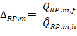
For each projected
future precipitation series ![]() , calculate the nonexceedance probability
, calculate the nonexceedance probability ![]() from the fitted GEV
from the fitted GEV ![]() . Find the corresponding quantile (
. Find the corresponding quantile (![]() at the GCM historical baseline by entering the value
of
at the GCM historical baseline by entering the value
of ![]() in the inverse CDF
in the inverse CDF ![]() . This is a scaling step introduced to incorporate the
future projections in the updated IDF, and uses the concepts of quantile delta
mapping (Olsson et al., 2009; and Cannon et al., 2015). The relative change
. This is a scaling step introduced to incorporate the
future projections in the updated IDF, and uses the concepts of quantile delta
mapping (Olsson et al., 2009; and Cannon et al., 2015). The relative change ![]() , is calculated using Eq. 22:
, is calculated using Eq. 22:
|
|
Eq. 20 |
|
|
Eq. 21 |
|
|
Eq. 22 |
(viii)
To generate the
projected future maximum sub-daily series at the station scale (![]() , use Eq. 19 by replacing
, use Eq. 19 by replacing
![]() to
to ![]() and multiplying by the relative change
and multiplying by the relative change ![]() from Eq. 22.
from Eq. 22.
|
|
Eq. 23 |
(ix) Generate IDF curves for the future sub-daily data and compare the same with the historically observed IDF curves to observe the change in intensities.
4.2 Updating IDFs for Ungauged Locations
The updating procedure for ungauged location IDF curves adopts a modified version of the equidistant quantile matching (EQM). The changes in future conditions due to climate change are captured from the GCMs by evaluating the magnitude and sign of change comparing the model’s baseline and future periods for each RCP and are applied to the ungauged IDF estimates from the gridded data. The flow chart of the modified EQM methodology is shown in Figure 6.

![]()

Figure 6: Modified Equidistance Quantile-Matching method for generating future IDF curves under climate change for ungauged IDF curves
The following section presents the modified EQM method
for updating the ungauged IDF curves that is employed by the IDF_CC tool
version 3. The following notation is used in the descriptions of the EQM steps:
![]() , stands for the annual maximum precipitation, j
is the subscript for 5min, 10min, 15min, 1hr, 2hr, 6hr, 12hr, 24hr sub-daily
durations, RP the return period in year, o the observed
historical series, h for historical simulation period (base-line for model
data), m for model (downscaled GCMs), f is the sub/superscript the
future projected series, p is the non-exceedance probability for a given
RP, F the CDF of the fitted probability GEV distribution and F-1
the inverse CDF. The steps involved in the algorithm are as follows:
, stands for the annual maximum precipitation, j
is the subscript for 5min, 10min, 15min, 1hr, 2hr, 6hr, 12hr, 24hr sub-daily
durations, RP the return period in year, o the observed
historical series, h for historical simulation period (base-line for model
data), m for model (downscaled GCMs), f is the sub/superscript the
future projected series, p is the non-exceedance probability for a given
RP, F the CDF of the fitted probability GEV distribution and F-1
the inverse CDF. The steps involved in the algorithm are as follows:
(i)
Extract the ungauged IDF
curves, representing the historical IDF, from the gridded dataset for all
durations (5min, 10min, 15min, 1hr, 2hr, 6hr, 12hr, 24hr) and all return
periods (2, 5, 10, 25, 50 and 100 years) ![]() at the selected location (UserMan: Section 3.2).
at the selected location (UserMan: Section 3.2).
(ii)
Extract daily maximums
for the historical baseline period from the selected GCMs (UserMan:
Section 3.2), ![]() .
.
(iii)
Fit the GEV probability
distribution to maxima series extracted fro the GCM series in (ii), ![]() .
.
(iv)
Extract daily maximums
from the RCP Scenarios (i.e., RCP 2.6, RCP 4.5, RCP 8.5) for the selected GCM
model (UserMan: Section 3.2), ![]() .
.
(v)
Fit the GEV probability
distribution to the daily maximums from the GCM model for each of the future
scenarios ![]() (UserMan: Section 3.2).
(UserMan: Section 3.2).
(vi)
For each projected
future precipitation series, calculate the quantiles (![]() using the non-exceedance
probability (
using the non-exceedance
probability (![]() for each RP (2, 5, 10, 25, 50 and 100 yeaers) from the
inverse CDF of the fitted GEV,
for each RP (2, 5, 10, 25, 50 and 100 yeaers) from the
inverse CDF of the fitted GEV, ![]() . Similarly, calculate the quantiles (
. Similarly, calculate the quantiles (![]() at the GCM historical baseline by entering the value
of the non-exceedance probability for each RP in the inverse CDF
at the GCM historical baseline by entering the value
of the non-exceedance probability for each RP in the inverse CDF ![]() . This is a scaling step introduced to incorporate
future projections in the updated IDF and mimics the concepts of quantile delta
mapping (Olsson et al., 2009; and Cannon et al., 2015). The relative change
. This is a scaling step introduced to incorporate
future projections in the updated IDF and mimics the concepts of quantile delta
mapping (Olsson et al., 2009; and Cannon et al., 2015). The relative change ![]() is calculated using Eq. 26, for each
R:P 2, 5, 10, 25, 50 and 100 years.
is calculated using Eq. 26, for each
R:P 2, 5, 10, 25, 50 and 100 years.
|
|
Eq. 24 |
|
|
Eq. 25 |
|
|
Eq. 26 |
(vii)
To generate the
projected future IDF curves for each duration and RP, at the selected location,
use ![]() and multiple by the relative change
and multiple by the relative change ![]() from Eq. 26.
from Eq. 26.
|
|
Eq. 27 |
5 Summary
This document presented the technical reference manual for the Computerized IDF_CC tool version 3 for the Development of Intensity-Duration-Frequency-Curves Under a Changing Climate. The tool uses a sophisticated, although very efficient, methodology that incorporates changes in the distributional characteristics of GCMs between the baseline period and the future period. The mathematical models and procedures used within the IDF_CC tool include: (i) spatial interpolation of GCM data using the inverse distance method; (ii) statistical analyses algorithms, which include fitting Gumbel and GEV probability distribution functions using method of moments and method of L-moments, respectively; and (iii) an IDF updating algorithm based on the EQM method. The document also presented step-by-step examples for the implementation of all the mathematical models and procedures used in the IDF_CC tool.
The IDF_CC tool’s website (www.idf-cc-uwo.com) should be regularly visited for the latest updates, new functionalities and updated documentation.
Acknowledgements
The authors would like to acknowledge the financial support by the Canadian Water Network Project under the Evolving Opportunities for Knowledge Application Grant to the third author for the initial phase of the project, and the Institute for Catastrophic Loss Reduction for continuous support of this project.
Allan, R.P., B.J. Soden, (2008) Atmospheric warming and the amplification of precipitation extremes. Science 321: 1480–1484.
Barnett, D.N., S.J. Brown, J.M. Murphy, D.M.H. Sexton, and M.J. Webb, (2006) Quantifying uncertainty in changes in extreme event frequency in response to doubled CO2 using a large ensemble of GCM simulations. Climate Dynamics 26(5): 489–511.
Bürger, G., T.Q. Murdock, A.T. Werner, S.R. Sobie, and A.J. Cannon, (2012) Downscaling extremes - an intercomparison of multiple statistical methods for present climate. Journal of Climate, 25:4366–4388.
Bürger, G., S.R. Sobie, A.J. Cannon, A.T. Werner, and T.Q. Murdock, (2013) Downscaling extremes - an intercomparison of multiple methods for future climate. Journal of Climate, 26:3429-3449.
Cannon, A.J., S.R. Sobie, and T.Q. Murdock, (2015) Bias Correction of GCM Precipitation by Quantile Mapping: How Well Do Methods Preserve Changes in Quantiles and Extremes? Journal of Climate, 28(17):6938-6959. DOI: 10.1175/JCLI-D-14-00754.1.
Cortes, C. & Vapnik, V. Mach Learn (1995) 20: 273. https://doi.org/10.1007/BF00994018
CSA (Canadian Standards Association), (2012) Technical guide: Development, interpretation, and use of rainfall intensity-duration-frequency (IDF) information: Guideline for Canadian water resources practitioners. Mississauga: Canadian Standards Association.
Faulkner, D.S., Prudhomme, C., (1998) Mapping an index of extreme rainfall across the UK Hydrology and Earth System Sciences, 2 (2-3), pp. 183-194
Gudmundsson, L., J.B. Bremnes, J.E. Haugen, and T. Engen-Skaugen, (2012) Technical Note: Downscaling RCM precipitation to the station scale using statistical transformations - a comparison of methods(link is external). Hydrology and Earth System Sciences, 16:3383–3390.
Hassanzadeh, E., A. Nazemi, and A. Elshorbagy, (2014) Quantile-Based Downscaling of Precipitation using Genetic Programming: Application to IDF Curves in the City of Saskatoon. J. Hydrol. Eng., 19(5): .943-955.
Hogg, W.D., D.A. Carr, and B. Routledge, (1989) Rainfall Intensity-Duration-Frequency values for Canadian locations. Downsview; Ontario; Environment Canada; Atmospheric Environment Service.
Hosking, J.R.M., and J.R. Wallis, (1997) Regional Frequency Analysis. Cambridge University Press, Cambridge.
Hosking, J.R.M., J.R. Wallis, and E.F. Wood, (1985) Estimation of the Generalized Extreme-Value Distribution by the Method of Probability-Weighted Moments. Technometrics, 27(3):251-261. DOI: 10.2307/1269706
Hunter, R.D., and R. K. Meentemeyer, (2005) Climatologically Aided Mapping of Daily Precipitation and Temperature . Journal of Applied Meteorology, 44:1501–1510,
Kao, S.C., and A.R. Ganguly, (2011) Intensity, duration, and frequency of precipitation extremes under 21st-century warming scenarios. Journal of Geophysical Research, 116(D16), D16119.
Kharin, V.V., F.W. Zwiers, X. Zhang, and G. Hegerl, (2007) Changes in temperature and precipitation extremes in the IPCC ensemble of global coupled model simulations. J Climate 20:1519-1444
Li, H., J. Sheffield, and E.F. Wood, (2010) Bias correction of monthly precipitation and temperature fields from Intergovernmental Panel on Climate Change AR4 models using equidistant quantile matching. Journal of Geophysical Research, 115(D10), D10101.
Mailhot, A., S. Duchesne, D. Caya, and G. Talbot, (2007) Assessment of future change in intensity-duration-frequency (IDF) curves for Southern Quebec using the Canadian Regional Climate Model (CRCM). Journal of Hydrology, 347: 197–210.
Maurer, E.P., and H.G. Hidalgo, (2008) Utility of daily vs. monthly large-scale climate data: an intercomparison of two statistical downscaling methods. Hydrology and Earth System Sciences, 12(2):551-563.
Maurer, E., H. Hidalgo, T. Das, M. Dettinger, and D. Cayan, (2010) The utility of daily large-scale climate data in the assessment of climate change impacts on daily streamflow in California(link is external). Hydrology and Earth System Sciences, 14(6):1125–1138.
Milly, P.C.D., J. Betancourt, M. Falkenmark, R. M. Hirsch, Z.W. Kundzewicz, D.P. Lettenmaier, and R.J. Stouffer, (2008) Stationarity Is Dead: Whither Water Management?, Science, 319(5863): 573-574.
Mirhosseini, G., P. Srivastava, and L. Stefanova, (2012) The impact of climate change on rainfall Intensity–Duration–Frequency (IDF) curves in Alabama. Regional Environmental Change, 13(S1):25–33.
Millington, N., S. Das and S.P. Simonovic, (2011) The Comparison of GEV, Log-Pearson Type 3 and Gumbel Distributions in the Upper Thames River Watershed under Global Climate Models. Water Resources Research Report no. 077, Facility for Intelligent Decision Support, Department of Civil and Environmental Engineering, London, Ontario, Canada, 53 pages. ISBN: (print) 978-0-7714-2898-2; (online) 978-0-7714-2905-7.
Nguyen, V.T.V., T.D. Nguye, and A. Cung, (2007) A statistical approach to downscaling of sub-daily extreme rainfall processes for climate-related impact studies in urban areas. Water Science & Technology: Water Supply, 7(2):183.
Olsson, J., K. Berggren, M. Olofsson, and M. Viklander, (2009) Applying climate model precipitation scenarios for urban hydrological assessment: A case study in Kalmar City, Sweden. Atmos. Res., 92:364–375, doi:10.1016/j.atmosres.2009.01.015.
Overeem, A., A. Buishand, and I. Holleman, (2007) Rainfall depth-duration-frequency curves and their uncertainties. Journal of Hydrology. 348(1-2):124-134. DOI:10.1016/j.jhydrol.2007.09.044.
Pacific Climate Impacts Consortium (PCIC) (2013) Statistically downscaled climate scenarios, https://pacificclimate.org/data/statistically-downscaled-climate-scenarios last accessed July 15, 2017.
Peck, A., P. Prodanovic, and S.P. Simonovic, (2012) Rainfall Intensity Duration Frequency Curves Under Climate Change: City of London, Ontario, Canada. Canadian Water Resources Journal, 37(3):177–189.
Piani, C., G.P. Weedon, M. Best, S.M. Gomes, P. Viterbo, S. Hagemann, and J.O. Haerter, (2010) Statistical bias correction of global simulated daily precipitation and temperature for the application of hydrological models. Journal of Hydrology, 395(3-4):199–215.
Sandink, D., S.P. Simonovic, A. Schardong, and R. Srivastav, (2016) A Decision Support System for Updating and Incorporating Climate Change Impacts into Rainfall Intensity-Duration-Frequency Curves: Review of the Stakeholder Involvement Process, Environmental Modelling & Software Journal, 84:193-209.
Simonovic, S.P., and D. Vucetic, (2012) Updated IDF curves for London, Hamilton, Moncton, Fredericton and Winnipeg for use with MRAT Project, Report prepared for the Insurance Bureau of Canada, Institute for Catastrophic Loss Reduction, Toronto, Canada, 94 pages.
Simonovic, S.P., and D. Vucetic, (2013) Updated IDF curves for Bathurst, Coquitlam, St, John’s and Halifax for use with MRAT Project, Report prepared for the Insurance Bureau of Canada, Institute for Catastrophic Loss Reduction, Toronto, Canada, 54 pages.
Simonovic, S.P., A. Schardong, D. Sandink, and R. Srivastav, (2016) A Web-based Tool for the Development of Intensity Duration Frequency Curves under Changing Climate, Environmental Modelling & Software Journal, 81:136-153.
Solaiman, T.A., and S.P. Simonovic, (2011) Development of Probability Based Intensity-Duration-Frequency Curves under Climate Change. Water Resources Research Report no. 072, Facility for Intelligent Decision Support, Department of Civil and Environmental Engineering, London, Ontario, Canada, 89 pages. ISBN: (print) 978-0-7714-2893-7; (online) 978-0-7714-2900-2.
Solaiman, T.A., and S.P. Simonovic, (2010) National centers for environmental prediction -national center for atmospheric research (NCEP-NCAR) reanalyses data for hydrologic modelling on a basin scale (2010) Canadian Journal of Civil Engineering, 37(4):611-623.
Solaiman, T.A., L.M. King, and S.P. Simonovic, (2011) Extreme precipitation vulnerability in the Upper Thames River basin: uncertainty in climate model projections. Int. J. Climatol., 31: 2350–2364.
Srivastav, R.K., A. Schardong, and S. P. Simonovic, (2014) Equidistance Quantile Matching Method for Updating IDF Curves under Climate Change, Water Resources Management, 28(9): 2539-2562.
Sugahara, S., R.P. Rocha, and R. Silveira, (2009) Non-stationary frequency analysis of extreme daily rainfall in Sao Paulo, Brazil, 29, 1339–1349. doi:10.1002/joc.
Taylor, K.E., R.J. Stouffer, and G.A. Meehl, (2012) An overview of CMIP5 and the experiment design. Bull Am Met Soc 93(4):485–498.
Walsh, J., (2011) Statistical Downscaling, NOAA Climate Services Meeting.
Werner, A.T., (2011) BCSD downscaled transient climate projections for eight select GCMs over British Columbia, Canada. Pacific Climate Impacts Consortium, University of Victoria, Victoria, BC, 63 pp.
Werner, A.T. and A.J. Cannon, (2015) Hydrologic extremes – an intercomparison of multiple gridded statistical downscaling methods. Hydrology and Earth System Sciences Discussion, 12:6179-6239,
Wilby, R.L., and C.W. Dawson, (2007) SDSM 4.2 – A decision support tool for the assessment of regional climate change impacts. Version 4.2 User Manual.
Wilcox, E.M., and L.J. Donner, (2007) The frequency of extreme rain events in satellite rain-rate estimates and an atmospheric general circulation model. Journal of Climate 20(1): 53–69.
Wood, A.W., L.R. Leung, V. Sridhar, and D.P. Lettenmaier, (2004) Hydrologic implications of dynamical and statistical approaches to downscaling climate model outputs(link is external). Climatic Change, 62:189–216.